The Manticore dataset
To characterize the voids in our Local Neighborhood, we use the Manticore-Local posterior realizations of the large-scale structure (McAlpine et al., 2025), a set of constrained N-body simulations initialized to be consistent with the galaxy positions identified in the 2M++ data compilation (Lavaux & Hudson, 2011).
Produced in the Bayesian framework of the BORG algorithm (Jasche & Wandelt, 2013), they represent 50 independent samples of the posterior distribution of the large-scale structure and allow us to carry out a complete statistical analysis of the voids.
A full description of the simulations can be found in McAlpine et al. (2025), and in the dedicated Manticore website.
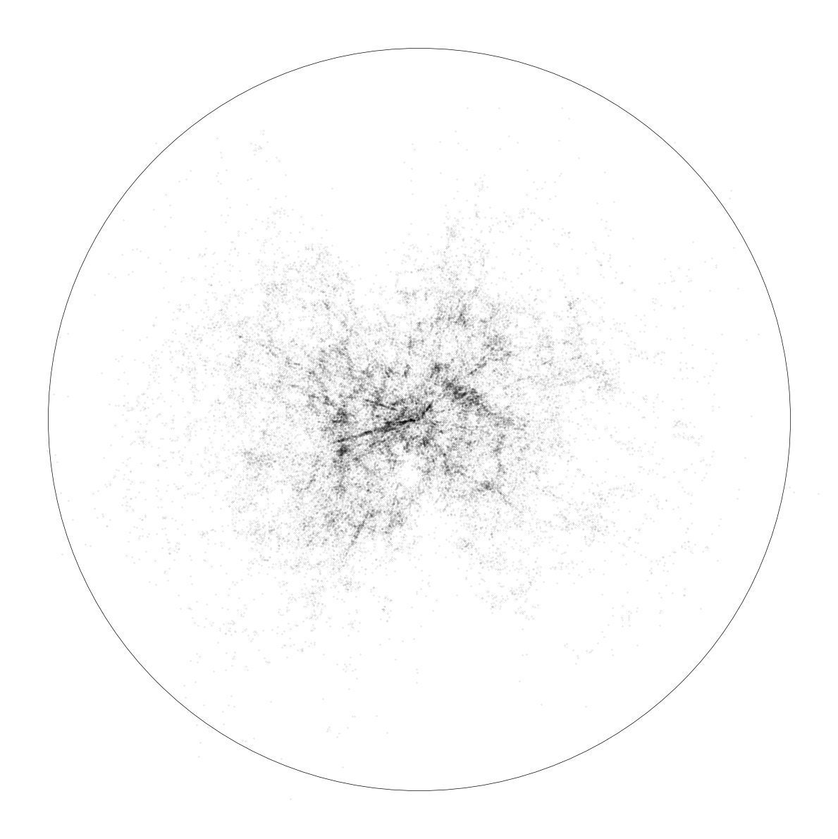
On the left we show the galaxy positions used for the inference, and on the right the corresponding set of 50 independent posterior realizations of halo distributions at present day. Stable structure can be recognized inside the dashed circle, corresponding to a $\approx 250 \, \text{Mpc} \approx 170 \, h^{-1} \ \text{Mpc}$ radius, i.e. the region where we have observations of galaxies. As there is no information to constrain the large-scale structure in the exterior part of the box, the density field is randomly distributed in this region.
 |
🠊 |  |
Void finding procedure
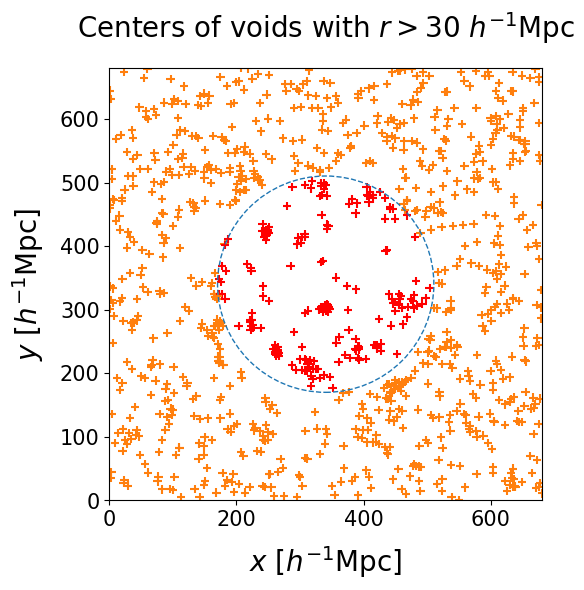
We run the VIDE void finding algorithm (Sutter et al. 2015) on each individual realization of the cosmic web. The resulting voids have complex morphologies, but they can be summarized with a center and an effective radius. In the left panel we select voids with $30 < r < 50 \ h^{-1} \, \text{Mpc}$, the crosses represent their centers and the circles correspond to their effective volumes. Despite some variations among different realizations, some regions of space are more likely to be identified as voids than others. The right panel shows a slice of the 3D space containing all void centers from all realizations. The points making up each cluster correspond to different samples of the same real void in the Universe.
Identifying stable voids in the posterior realizations of the Universe reduces to a detection problem. We perform a posterior clustering analysis to identify high-significance voids: the details of the clustering strategy and the posterior distribution estimation are illustrated here.
 |
 |
Bayesian catalog and posterior distributions
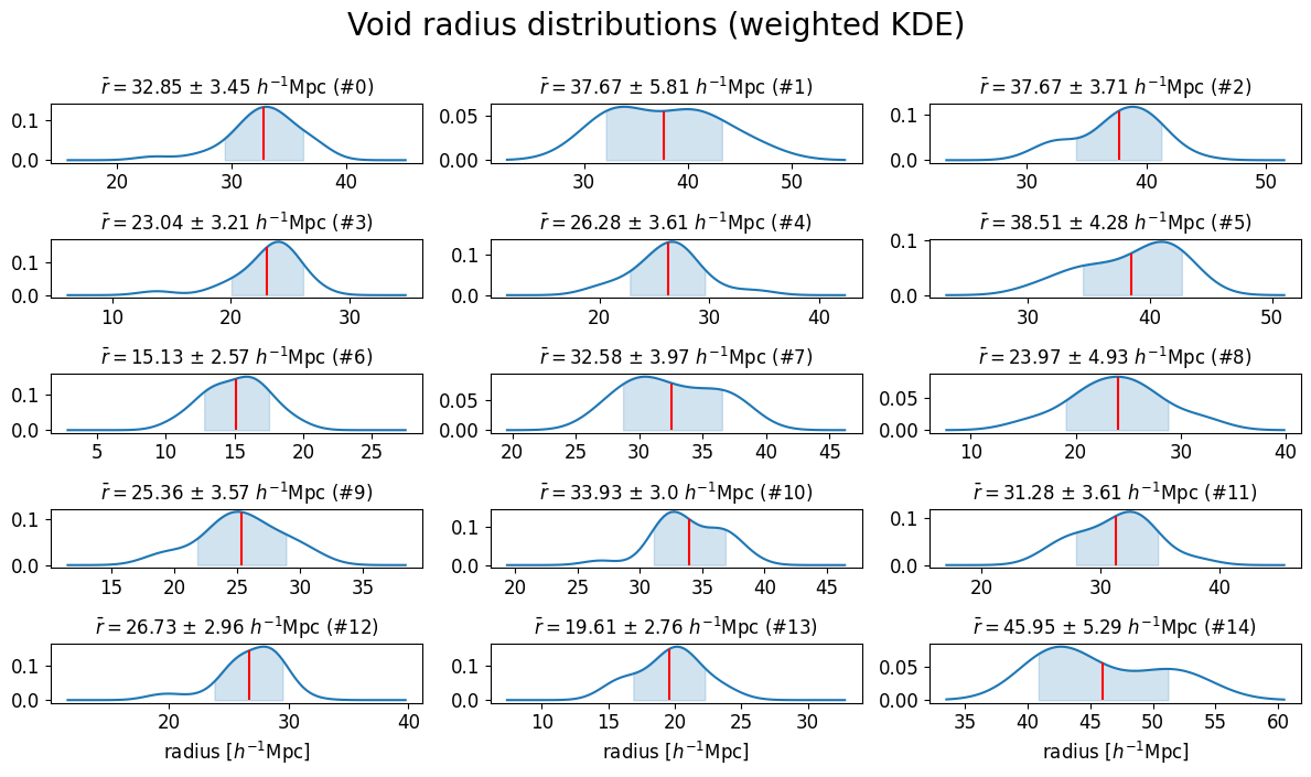
We produce a catalog of 100 high-significance cosmic voids in the neighboring Universe, up to a distance of $\approx 200 \, h^{-1} \, \text{Mpc}$. The Bayesian nature of our procedure provides us with probability distributions for the quantities of interest, allowing rigorous uncertainty quantification. The following figures represent the posterior distributions of void centers, and a selection of the posterior distributions of the void radii (the full plot can be found here).
Our catalog features a rigorous uncertainty quantification: a table summarizing the main quantities of interest can be found in the VoidGallery section of this website. In order to visualize voids, we can consider the mean posterior of both distributions, effectively approximating them as spheres with well-defined centers and radii. The result is presented here, with the colorscale representing the redshift. The zone of avoidance of galaxy surveys corresponding to the galactic plane produces a visible region with fewer voids.
The actual shape of voids
The VIDE void finder performs a Voronoi tessellation on the tracers of the density field and merges the resulting cells with a watershed transform. As a result, void morphologies are very complex. We show the individual contributions to a single statistical void: samples from different realizations are represented through circles corresponding to the Voronoi cells making an individual void, while the black cross and circle represent their mean centers and effective radii. Finally, the yellow star and circle represent the mean posterior of the center and radius, as inferred from our clustering procedure.
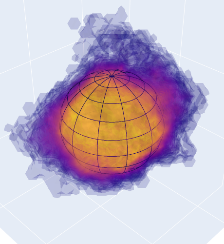
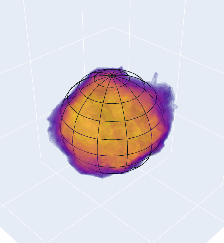
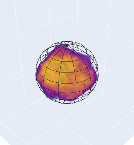
To characterize the shape of the void, we grid the space around the void center, and count how often a particular point is contained in a Voronoi cell. We define the Voronoi overlap rate, a quantity ranging from zero to one after appropriate normalization, which describes the environment around the void center. Higher values correspond to the most underdense parts of the void, while lower values define the boundaries. The left panel shows this function - which we name Voronoi cloud - overimposed to a wireframe sphere of effective volume. The volume of the full cloud exceeds the statistical one, as the farther outskirts are labeled as void only in a few realizations, but are unlikely to be part of the void. Appropriate truncations of this cloud can either yield the mean posterior volume (center panel) or probe the deeper interior of the void (right panel). Further details on the Voronoi clouds and how we perform the truncation can be found here
| Full cloud | Volume conservation | Void interior |
|---|---|---|
 |
 |
 |
Finally, we show a fully interactive plot of the Voronoi cloud of an example void, as well as the galaxies used in the inference. The spherical approximation loses information on the full shape of voids, while the Voronoi cloud provides a well-defined template for underdense environments.
Do our voids match the underlying halo field?
We compare our voids to the average of the 50 posterior realizations of the underlying halo field. In the left panel we marginalize the Voronoi cloud by summing its values over the $z$ direction. We plot the $0$ and $0.5$ contour levels of the renormalized marginal over a slab of the halo field, with thickness equal to void radius. We find that the contours follow the density profiles. However, this 2D projection loses the full three-dimensional information: on the right panel we show different slices in $z$, which highlight the relation between the void and its environment.